Introduction
A. The Need for Tactile Sensors
Giving robots the sense of touch is a key challenge in robotics to enable manipulation of objects with human levels of dexterity [1]. To complement vision sensing, robots require tactile sensors providing measurements of the normal and tangential forces at the points of contact [2]. The contact information enables force control and slip detection strategies allowing the manipulation of fragile objects. The force measurements can also be used to estimate the weight of unknown objects prior to a precision task [3]. Contact detection is also critical for a smooth and safe interaction with human [2].
Based on the tactile sensing capabilities of humans, technical design targets for tactile sensors were derived in [4], with the integration aspects elaborated later in [5]. The key performance targets are: sub-cm spatial resolution (e.g. pitch of 5 mm in the palm), 3D force vector sensing, 1 g-weight resolution (10 mN), 1:1000 dynamic range, 1-ms response time. A low non-linearity and hysteresis are also required but not quantified in [4], but we assume below a few percents. The sensor contact surface should be compliant to increase the contact area, and have a skin-like feeling. This excludes stiff sensors. For example, the 6D force/torque sensors in [6] and [7] based on strain gauges and variable capacitors respectively. Such sensors are better suited for measuring the force and torque at the joints (as opposed to the contact at the skin surface).
B. Technologies for Tactile Sensing
An extensive review of the alternative technologies for tactile sensors is available in [8]. Here, we restrict the discussion to tactile sensors that have been integrated into robotic hands or fingers.
A liquid metal tactile sensor is demonstrated in [9]. The resistance of a liquid metal flowing in microfluidic channels is modulated by the external forces. Such sensor is highly stretchable, and can be incorporated all around the robot fingertips. The downside is that the sensor is not a localized 3D force sensor. Instead, the distributed forces are mapped to a resistance change. By combing multiple sensors (one per fingertip in the above reference), a pattern emerges. This is then better suited to specialized classification task after dedicated training. The above reference provides an example of texture recognition to differentiate among 10 possibilities. BioTac [10] is a commercial product also based on a fluid in microchannels, but this time with a pressure sensor. Again this does not measure the localized 3D contact force.
Another approach is to use a high-end optical camera that can measure the localized micrometer deformation of an elastomer. This technology is commercially available under the name Gelsight. Such sensors have been recently integrated into a smart multi-modal robotic gripper [11]. The NeuroTac is also a camera-based sensor. It was also demonstrated in a robotic hand to recognize objects [12]. In both of these examples, the camera consists of a substantial pixel array (320x240 for Gelsight) transmitted at video rate for further analysis. This stretches the communication bandwidth and power consumption.
A leaner approach is demonstrated in [13]. The optical sensor OptoForce OMD-10 [14], now discontinued as a standalone commercial component, is used. A quadrant of photodiode detectors is used—not a full camera. A light source shines a light into an elastic dome from the inside. The deformation of the dome due to the contact forces is sensed by the detectors. Power consumption is rated at 240 mW. This is several times larger than the consumption of typical 3D magnetometers, which are covered next.
C. Magnetic Force Sensors
Magnetic force sensors rely on a compact single-chip 3D magnetometer measuring the displacement of a magnet embedded in an elastomer as illustrated in Fig. 1. In [15], the 3D sensing capability of such transducing scheme were demonstrated—with competitive resolution of 1.42 mN in normal force and 0.71 mN in shear forces. The same authors [16] later incorporated four such sensors in a low-cost 2x2 array, named MagTrix, with 6-mm pitch. Even larger arrays have been demonstrated based on the same principle by other groups: 4x4 in [17], and 24 sensors in [18] covering a fingertip with a distributed magnetic skin, and later integrated in the iCub robot [19]. This demonstrated the unique advantages of the magnetic force sensors: 3D force sensing in a compact and cost-effective package with just one chip per tactile pixel (”taxel” in the literature: TActile piXEL). Others have extended this technology further. A continuous magnetic skin of 15 mm2 (consisting of magnetic microparticles) was demonstrated in [20]. Sub 1-mm “super-resolution” was achieved in [21] by combining an array of magnetic force sensors, sinusoidal magnetization of a flexible film, and deep learning.

Magnetic force sensors. All sub-figures cropped from [15] (license: CC BY 4.0) apart from the inset. (a) Cross section illustrating the force-to-magnetic-field transducing mechanism. (b) 3D schematic of the sensor. Inset: MLX90393 magnetometer micrograph with the sensing spot in blue. (c) Sensor operation close to its resolution limit.
All the previously-cited magnetic force sensors [15]–[16][17][18][19][20][21] rely on the same magnetometer chip: the MLX90393 [22] from Melexis. It is a single-pixel 3D magnetometer. The integrated circuit micrograph is shown in the inset of Fig. 1(b). Note the position of the single magneto-concentrator highlighted in light blue at the chip center. This nickel and iron film bends the magnetic field lines parallel to the chip surface. The resulting normal field lines are redirected to the Hall plates in the integrated circuit. Via proper sign combinations between the Hall plates, 3D vector sensing of the local magnetic field is achieved. In this concept, each tactile pixel (”taxel”) corresponds to a single magnetic pixel.
This concept is overly sensitive to magnetic stray fields. The sensor cannot distinguish the signal from the possible stray-field disturbances. This is a critical issue as in the real world there is no guarantee that the robotic hand will be shielded from magnetic stray fields. The Earth’s magnetic field ≈50μT, or a field arising from a nearby electrical motor to actuate the robot, or other unrelated nearby magnet, directly leaks into the signal path of each taxel, thereby corrupting the force readout.
An inductive-based sensor was proposed in [23] to reject low-frequency magnetic stray fields. The 3D force is transduced into Eddy currents flowing in pick-up coils at a few MHz. This scheme is insensitive to low-frequency magnetic stray fields. The drawbacks are the large footprint (larger than 1 cm) of the coils on the printed circuit board (PCB) and the parasitic sensitivity to stray metals.
A magnetic force sensor, preserving the strengths of the previously-cited ones [15]–[16][17][18][19][20][21], while exhibiting stray-field immunity is desirable. This is what we propose here.
The paper is structured as follows. In Section II, we first describe the multi-pixel concept and its built-in rejection of stray fields. The experimental characterization results are presented in Section III. In Section IV, the sensor is integrated into a robotic hand for a real-world demo. We discuss our results, and benchmark them against the state of the art in Section V.
Sensor Design
A. Gradiometric Concept
We propose a magnetic force sensor with multiple nearby pixels inside the same integrated circuit (IC) package. As shown in Fig. 2(a), this solution addresses the issue of stray fields generated from nearby conductors, magnets or motors. The pior-art sensors, based on a single 3D magnetometer, can be corrupted whereas the multi-pixel approach allows a differential measurement depicted in Fig. 2(b). We repurposed the MLX90372 linear-displacement sensor [24], [25]. This sensor usually outputs the angular displacement along an arc. Here, we configured the chip in test mode, and directly accessed the raw magnetic readouts of the individual pixels from the memory. A single TSSOP package (5x4.3x0.9 mm3) contains two side-by-side CMOS dies, with two pixels per die. Hence, in one compact package, there are four magnetic pixels (separated by only ≈2 mm). This enables the measurement of the gradient of the magnetic field (with components of the form ∂Bi∂xj) in the millimeter scale. Each pixel senses the normal component of the field Bz and the Bx in-plane component. The By component would be helpful, but is not available in this sensor.
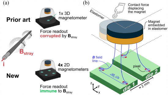
Diagrams showing the concept of the multi-pixel magnetic force sensor. (a) Comparison with prior-art sensors. (b) Magnetic field lines and differential sensing in multi-pixel magnetic force sensor–this scheme is immune to stray fields.
Like in the prior art, the IC package is then covered by a soft elastomer in which a disk magnet with axial magnetization is embedded. Thanks to its elasticity, the elastomer is deformed by the contact force applied, thereby displacing the magnet. This modulates the magnetic field pattern, which is sensed at four locations by the four magnetic pixels.
Normal and lateral displacements are sensed by the magnetic sensor. For a normal displacement of the magnet, the gradiometric component ∂Bx∂x is the most impacted. Conversely for a lateral displacement, the impact is mostly on the gradiometric component ∂Bz∂x. Fig. 3 shows the four different sensed Bz signals when displacing the magnet laterally in every direction in the XY plane. The signal strength at one pixel naturally increases as the magnet gets just above this pixel. Note that the heatmaps in Fig. 3 are plotted in terms of displacement, not yet the force. A force calibration, which is covered later, is required to extract the force vector.
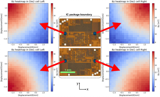
Principle of operation when sensing a later displacement. Outside: heatmap of the 4 Bz signals as a function of the lateral displacements in the XY plane. Center: micrograph of the side-by-side CMOS dies.
B. Elastomer and Magnet
In the prior art, the elastomer shape was either a pyramid [26] or a dome [15]. We selected here a cylinder with a flat contact surface, as opposed to a tip, to minimize the magnet tilt and offer a compliant surface that can wrap around objects–a cuboid would be a valid alternative. As in the two papers cited above, the neodymium magnet is embedded inside the elastomer (Dragon Skin 20 from Smooth-On) to avoid direct contact with ferromagnetic materials.
The key design tradeoff is between the signal-to-noise ratio (SNR) and the full-scale force. Together they also set the minimum resolvable force. Table I compiles our optimized design parameters for our prototype targeting robotic hands and grippers with a full-scale force ≳2 N. This level of maximum force (2 N) was, for example, reported in the robot Vizzy’s fingertips during the manipulation of fragile objects [3].
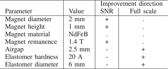
The size of the magnet and its remanence are directly related to the magnetic signal amplitude. Therefore, a bigger stronger magnet improves the signal-to-noise ratio (SNR), with little impact on the full-scale force. A smaller airgap improves the SNR. However, it also limits the physical displacement, and hence the full-scale force. The elastomer hardness is also subject to the same tradeoff. A harder elastomer enables a larger full-scale force. However, for the same force applied, the displacement of the magnet will be smaller compared to a softer material. This means that increasing the hardness also reduces the change of magnetic signal, hence the SNR. Finally, the elastomer diameter acts as a scaling factor between the overall force and the localized pressure just above the magnet. A larger diameter dilutes the force over a larger area thereby lowering the SNR, while accommodating larger full-scale force. Fig. 4 shows photographs of the complete sensor realization assembled on a PCB.

C. Signal Chain
Fig. 5 depicts the functional block diagram of the signal chain. The corresponding mathematical operations are described in the appendix. The 8 digital output signals of the chip, are first scaled by a quadratic temperature compensation based on the readout of the temperature sensor in the chip. This is to correct for the sensitivity drop of the Hall effect with increasing temperature (−0.5%/∘C).

Functional block diagram of the force/torque (F/T) sensing signal chain. The 8 magnetic signals and the temperature are acquired and converted on chip to digital values, which are further processed off chip.
The stray magnetic fields are then rejected by using combinations of field components where the mean of Bx field and Bz field are first removed. The remaining terms are related to the gradient of the magnetic field B⃗ . More precisely, to its finite-difference approximation ΔB⃗ over the millimeter scale: ∂Bx∂x≈ΔBx/Δx and the other in-plane differences. In other words, the force sensor algorithm processes the magnetic field differences within the two dies.
The feature augmentation block corresponds to the addition of the norm B2x+B2z−−−−−−−√ in each sensing pixel. We obtain a vector signal of dimension 12: {Bx,Bz,Bnorm} at each pixel.
The last step consists in generating a new vector containing all second-order polynomial combinations of the 12-dimensional vector, including interaction terms. Eventually, the signal obtained after this process is a vector of dimension 91. In the current prototype, the signal processing is executed off chip, and the numerical complexity is not a constraint.
To obtain the final force and torque, a 91-by-5 weight matrix multiplies the processed signal. The resulting vector of dimension 5 contains the 3 forces and 2 planar torques. The vertical torque component is not sensed in this device because of its insensitivity to vertical rotation (due to the symmetry of the magnet). The weights are obtained through a training procedure described in the next section.
Experimental Results
A. 3D Force Calibration
The training data set used to calibrate the model (ie. find the weight of the inference matrix), is obtained with a reference load cell (ATI nano17) mounted on a 3-axis moving platform. For each new training data, the platform moves according to the desired 3D displacement vector, thereby stressing the top surface of the elastomer. Both the force from the load cell and the magnetic signals from the sensor are measured and saved. In between each step, the platform always moves back to a resting position to let the elastomer recover its original shape. We collected the training data corresponding to 13’000 positions in random order. The various positions are based on a comprehensive sweep over the cylindrical coordinate system with depth up to 1.5 mm and radius up to 1.1 mm. The calibration setup is shown in Fig. 6(a). The weight matrix was trained on this data set, optimizing its components based on a stochastic gradient descent algorithm with the Huber loss function and a L1 regularization term.

Force calibration setup (showing the sensor, the load cell, and the moving platform) and model regression. (a) Force calibration setup. (b) Normal force and (c) shears forces predicted by the algorithm. (d) In-plane predicted torques.
Fig. 6(b),(c) show the matching between the forces measured by the calibration setup and the forces predicted by the algorithm. The coefficients of determination evaluated here (R2) are 0.996 (Fz), 0.966 (Fx) and 0.949 (Fy) which are all close to 1. Hence, there is a good correlation between predicted and measured values: the regression is accurate for all 3 dimensions. Likewise, the torque components predicted (Tx and Ty) correlate well with the torque measured by the calibration setup (see Fig. 6(d)).
B. Force Resolution
We focus now on the key performance parameters for normal force sensing. The noise is dominated by the thermal noise arising from the Hall plates resistance (≈4 kΩ). We described the signal conditioning electronics in [27]. The input-referred magnetic noise is approximately 9μT at 160∘C, and about three times smaller at room temperature with a time constant of around (τ≈220 μs). In the present paper, each magnetic measurement is averaged four times to obtain an equivalent time constant around 1 ms in line with the target application (ref. [4] mentions a response time target of 1 ms).
To characterize the resolution, the standard deviation was extracted from a set of 2000 force measurements without load (Fz=0). Fig. 7 depicts the empirical probability density function yielding a RMS force resolution of around 2.7 mN. This is better than the design guidelines in [4] and competitive with prior-art magnetic force sensors that are not stray-field immune. This is remarkable as stray-field immunity comes with a penalty in terms of the SNR, because of the limited magnetic field differences over the surface of an IC. This penalty is here mitigated by the multi-pixel combination enhancing the SNR.
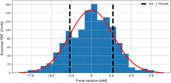
Empirical probability density function (PDF) of 2000 normal force measurements in unloaded condition (Fz=0) at room temperature. The measurements were mean corrected such that they represent the variations around the mean. The magnetic measurements were also averaged off-line four times to emulate a 1-ms sensor time constant.
C. Stray-Field Immunity (SFI)
To quantify the impact of uniform external fields on the sensor readout, the prototype was placed between two Helmholtz coils generating ±2 mT as shown in Fig. 8(a). Such a field is for example found at 3 cm of common home appliances [28]. With the gradiometric concept, the force measured by the sensor is not impacted by the external applied field as seen in Fig. 8(b). The stray-field error is limited to 0.3% of the full scale (Fig. 8(b), blue curve). The prototype was re-configured to operate as a plain magnetometer without stray-field rejection. This emulated the prior-art sensors. The stray field leaks directly into the signal path without any rejection, and the error is almost two orders of magnitude larger (20% at −2 mT, Fig. 8(b), red curve).

Stray-field verification. (a) Setup used. The picture shows an applied stray field in the x direction, but the sensor can be rotated to emulate an arbitrary-oriented stray field. (b) Stray-field error with and without the rejection algorithm.
D. Thermal Drift
To investigate the impact of a temperature change, a thermal setup was developed using a thermostream. The thermostream is flowing air at a controlled temperature into a thermally-insulated box containing the prototype. A tip linked to the reference force sensor (ATI nano17) applies a normal force inside the box. A non-direct contact solution was chosen as the reference force sensor must be kept at room temperature. Several normal push experiments were performed at different temperatures ranging from 0 to 50∘C. These experiments showed that the normal forces measured by the ATI nano17 varied with the temperature. In Fig. 9(a), it can be seen that for the same amplitude of the magnetic signal readout, the force drifted significantly over the temperature range. As an example, for a 25 mT readout, the measured force varied from 1.3 N to 1.6 N.
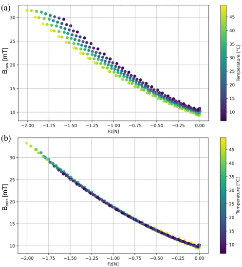
Magnetic response over temperature. The color represents the temperature in ∘C measured by the on-chip temperature sensor. (a) Without thermal correction. (b) With thermal correction.
The root cause of the force drift over the temperature range is the thermal expansion of the elastomer. This conclusion is based on the following observations. (1) Without any external force applied, the elastomer height is varying with the temperature (contraction or expansion), resulting is a change of the distance between the magnet and the Hall plates. (2) The physical properties of the elastomer are changing with the temperature, resulting in a change of stiffness. To address these effects, a thermal correction was proposed with the following form:

where ΔT=(Tchip−35∘C) is the temperature deviation measured by the on-chip temperature sensor calibrated at 35∘C. This form corresponds to a first-order correction with slope and offset. Physically, α is a constant capturing the change in the elastomer hardness, and β is a constant compensating the change in the elastomer height. Both constants, α and β, were tuned manually. Fig. 9(b) shows that, after thermal correction, the sensor’s force readings have minimum variation over temperature.
Integration in Robotic Hand
The force sensor was mounted on a commercial robotic hand (qb SoftHand from qbrobotics). A basic force control algorithm was implemented to have the hand grasp gently a balloon. Fig. 10 depicts the demonstration setup.

Demonstration of the effect of magnetic stray fields on a robotic hand with force sensor feedback. The stray field at the sensor is about 3 mT in this configuration. (a) The multi-pixel sensor rejects the stray field coming from the nearby magnet, and the force is well regulated. The hand keeps hold of the balloon with the proper force. (b) On the contrary, the sensor with the legacy single-pixel concept is corrupted: the hand wrongly releases the balloon. (c) Block diagram of the closed-loop control algorithm.
Using the sensor as a single-pixel plain magnetometer, the force is initially well regulated in the absence of stray-field disturbance—this is like the prior-art sensors. When approaching a magnet though, the force sensor is corrupted by the stray field. Consequently, the hand either releases or crushes the balloon, depending on the polarity of the approaching pole.
On the contrary, when using the multi-pixel concept, the force sensor is not perturbed by the approaching magnet. The force remains properly regulated regardless of the approaching magnet (down to distance of a few centimeters). A video of the experiment is available in the supplementary materials.
Conclusion
To put our results into perspective, Table II compares them against other force sensors realized in different technologies mentioned in the introduction. The recent magnetic force sensor [29] achieves 3D force vector sensing, state-of-the-art resolution and compactness (with four sensors integrated in each finger of the Vizzy robot), but the sensitivity to stray fields remains a key limitation. Our prototype remains competitive in terms of resolution and size while addressing this limitation: only a minor fraction of the stray field leaks.

The optical sensors are naturally fully immune to magnetic stray fields. They also offer similar 3D force sensing performance. See for example the OptoForce sensor [14]. It is a excellent functional fit for robotic hand integration as demonstrated in [13]. However, the discrete optical components drive the cost upwards. Before its obsolescence, it was available from distributors for several hundreds of dollars—this is a premium sensor (now available as a bulkier module). In contrast, ReSkin from Facebook AI is an open-source 20mm-by-20 mm tactile skin based on magnetic technologies that can be made for just $6 [31], [32]. Once again, the sensitivity to stray fields remains a key limitation.
As an example of another compact and cost-effective sensor, consider the commercially-available MicroForce Sensors FMA Series from Honeywell [30]. It is based on piezo-resistive technology, with a small form factor (the size of an IC package). It achieves competitive force resolution, but crucially it only senses the normal force.
As a conclusion, our prototype exploits the known assets of magnetic force sensors: 3D force vector sensing, softness, cost-effectiveness and compactness. Our multi-pixel concept makes the sensor robust to real-world parasitic stray fields. Our work has advanced the robustness of force sensing for robotic applications.
This appendix provides the mathematical formulation of the signal chain. Each block is mathematically formulated as a transfer function relating its output Y to its input X. The dimensions of these vectors are indicated in Fig. 5.
Sensitivity correction (in/out: raw/corrected fields)
View Source

Mean removal (out: field differences)
View Source

Feature augmentation (out: extra features)
View Source

Polynomial augmentation (out: final features)
View Source

Inference (out: 3D force and 2D torque)